# Preliminary imports

import tabulate
from pprint import pprintThis semester I have been teaching a course called “Statistical Programming for Ancient World” study. As a result I have been returning frequently to some natural language processing fundamentals from Manning and Schütze’s 1999 book Foundations of Statistical Natural Language Processing (Manning and Schütze (1999)) and have been thinking that it may be useful to computational philologists just starting out for me to work through this book using Latin or Ancient Greek examples. This is the first notebook in this series and looks at FSNLP 1.4.2 on “Word counts”.
What we want to do here is represent a Latin text—and we will start by representing a text as a list of words and then count the words to determine which are the most frequent. Manning and Schütze used Tom Sawyer for this exercise. We’ll use Cicero’s In Catilinam. A word count like this is the most basic of text analysis tasks, but it is still one of the most useful. The FSNLP example, shown in Table 1.1, also shows the “Use”, that is roughly the part of speech of each of the items listed.
Pseudocode for FSNLP 1.4.2
- Load our library of Latin texts, keeping only In Catilinam
- Get the tokens for the text.
- Count the tokens, ranking them from most to least frequent and keeping only the top 15.
- Add the word counts to a table with the columns “Word”, “Freq.” and “Use”
Workflow
As always, we start with our basic imports…
…and set up our corpus reader and pull out the texts we want to describe.
# PC 1: Load our library of Latin texts, keeping only *In Catilinam*

from latincyreaders import TesseraeReader

T = TesseraeReader()

file = 'cicero.in_catilinam.tess'
cicero = T.fileids(match=file)
pprint(cicero)['cicero.in_catilinam.tess']We can then use our corpus reader to get a list of the tokens in this text. Reminder that the output here will be a generator of spaCy Token objects (as annotated by the LatinCy pipeline). We convert this to a list for ease of reference. The advantage of using these Token objects—instead of plaintext words—is that they have POS tags available, which we can then use for the resulting table. So, below we see the first word in In Catilinam along with its Python type, i.e. the spaCy Token object.
# PC 2: Get the tokens for the text

tokens = list(T.tokens(fileids=cicero))

for i, token in enumerate(tokens, 1):
    print(f'{i}: {token} {type(token)}')
    break
1: quo <class 'spacy.tokens.token.Token'>Let’s now extract only the annotations that we plan to use for the table, namely the text of the token and its POS tag. Here we see these annotations for the first ten tokens in our text.
tagged_tokens = [(token.text, token.pos_) for token in tokens]

data = []

for i, (word, tags) in enumerate(tagged_tokens[:10], 1):
    data.append((word, tags))

print(tabulate.tabulate(data, headers=['Word', 'Tag']))
Word Tag
--------- -----
quo ADV
usque ADV
tandem ADV
abutere VERB
, PUNCT
Catilina PROPN
, PUNCT
patientia NOUN
nostra DET
? PUNCTNow we can use the Counter class from the collections module to count the token texts, excluding non-alphabetic tokens (like punctuation) from the results. (How we make such preprocessing decisions will be the subject of a future notebook.) When we pass a Python list to Counter, we get an dictionary-like object that takes unique list items for its key and the number of time this item appears in the list as the value. For example, the word et appears 259 times in In Catilinam and so would be represented in our Counter as…
{
‘et’: 259
}
And Counter has a most_common method that returns a list of tuples where the first element is the key (the word) and the second element is the value (the count), reverse sorted by count. We see below the first fifteen (15) items in such a “most common” list for our text.
# PC 3: Count the tokens, ranking them from most to least frequent and keeping only the top 15.

from collections import Counter

# Count the tokens

counter = Counter(token.text for token in tokens if token.text.isalpha())

# Get the 15 most common tokens
top_15 = counter.most_common(15)
print(top_15)
[('et', 259), ('in', 235), ('non', 205), ('atque', 142), ('qui', 141), ('ad', 137), ('esse', 135), ('que', 134), ('est', 132), ('ut', 120), ('cum', 119), ('si', 113), ('quod', 104), ('ac', 91), ('a', 87)]We can combine the data from the last few cells to combine our list of most frequent words with the all relevant POS tags. Note for example that word et in this text appears as both a conjunction and an adverb. We can use the defaultdict class to keep track of data: the word_tags variable keeps a dictionary where the words are the key and the value is set of observed POS tags. See below for an example based on the word et.
# Get all of the possible tags for each type

from collections import defaultdict

word_tags = defaultdict(set)

for token in tokens:
    if token.text.isalpha():
        word_tags[token.text].add(token.pos_)

# Print the tags for the top 15 tokens
for word, count in top_15[:1]:
    print(f'{word}: {count} {word_tags[word]}')
et: 259 {'CCONJ', 'ADV'}Finally, we put this all together in a table (using tabulate) with the columns from SFNL 1.4.2. The table is shown below.
# PC 4: Add the word counts to a table with the columns "Word", "Freq." and "Use"

data = []

for word, count in top_15:
    tags = word_tags[word]
    data.append((word, count, ', '.join(tags)))

print(tabulate.tabulate(data, headers=['Word', 'Freq.', 'Use']))
Word Freq. Use
------ ------- -----------
et 259 CCONJ, ADV
in 235 ADP
non 205 PART
atque 142 CCONJ
qui 141 PRON
ad 137 ADP
esse 135 AUX, NOUN
que 134 CCONJ
est 132 AUX
ut 120 SCONJ, ADV
cum 119 SCONJ, ADP
si 113 SCONJ
quod 104 SCONJ, PRON
ac 91 CCONJ
a 87 ADPWe can also make one additional refinement. In the FSNLP example, “Use” is spelled out a bit more than our POS tags. We can take advantage of spaCy’s tag mapping to expand our uses.
# PC 4 (extra): Map the tags to their definitions using spaCy's explain
import spacy
# Update the table with spaCy's built-in explanations
data = []
for word, count in top_15:
tags = word_tags[word]
# Map each tag to its explanation using spacy.explain()
mapped_tags = ', '.join(spacy.explain(tag) for tag in tags)
data.append((word, count, mapped_tags))
print(tabulate.tabulate(data, headers=['Word', 'Freq.', 'Use']), end="\n\n")
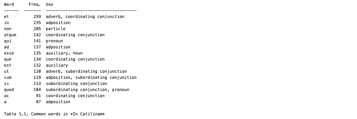
print("Table 1.1. Common words in *In Catilinam*")Word Freq. Use
------ ------- -------------------------------------
et 259 coordinating conjunction, adverb
in 235 adposition
non 205 particle
atque 142 coordinating conjunction
qui 141 pronoun
ad 137 adposition
esse 135 auxiliary, noun
que 134 coordinating conjunction
est 132 auxiliary
ut 120 subordinating conjunction, adverb
cum 119 subordinating conjunction, adposition
si 113 subordinating conjunction
quod 104 subordinating conjunction, pronoun
ac 91 coordinating conjunction
a 87 adposition
Table 1.1. Common words in *In Catilinam*With this we have accomplished our FSNLP goal of answering “What are the most common words in the text?” Moreover, just like the Tom Sawyer list, it is primarily taken up with the “little words…which have important grammatical roles.” So, the prepositions (or adpositions as they are called in the spaCy space), the conjunctions, the particles. We a few pronouns and other part of speech as well. (We also have an error—esse shouldn’t ever by a NOUN, but remember that the LatinCy tagger works at around 97% accuracy, so we should expect some errors.)
What we don’t have in this list is a “Tom”. That is, Manning and Schütze note that “Tom” appears in the top 15 words of Tom Sawyer. Whereas most of the words reflect general patterns of English usage, “Tom…clearly reflects the text that we chose.” For In Catilinam we have to go a bit further into the frequency list, but we do see that proper nouns like Quirites and forms of Catilina appear in the top 100 words of this text though would be unlikely to appear in the top 100 words of a different Latin text. We can say that the former are “representative” of the Latin corpus and the latter are not. This is an idea that we will continue to revisit as we describe the language and its texts from the FSNLP perspective.
top_words = counter.most_common(100)

data = []
for i, (word, count) in enumerate(top_words, 1):
    tags = word_tags[word]
    # Map each tag to its explanation using spacy.explain()
    mapped_tags = ', '.join(spacy.explain(tag) for tag in tags)
    if "proper noun" not in mapped_tags:
        # Skip proper nouns
        continue
    data.append((i, word, count, mapped_tags))

print(tabulate.tabulate(data, headers=["Rank", 'Word', 'Freq.', 'Use']), end="\n\n")
print("Table 1.2. Rank of proper nouns in the top 100 words of *In Catilinam*")
Rank Word Freq. Use
------ --------- ------- -----------
37 Quirites 39 proper noun
38 Catilina 37 proper noun
80 Catilinam 19 proper noun
Table 1.2. Rank of proper nouns in the top 100 words of *In Catilinam*Word counts are a fundamental—perhaps the fundamental task of text analysis. They are a straightforward, easy-to-explain representation of a text and much of what we will do in future notebooks will be variations on a counting theme and in the FSNLP notebooks in particular they will be statistical variations on this theme in particular.
References
Manning, C. D., and H. Schütze. 1999. Foundations of Statistical Natural Language Processing. Cambridge, MA: MIT Press.
Originally published April 15, 2025.
Updated February 2, 2026 to use the latincyreaders package (v1.0.2), which replaces the deprecated cltkreaders package.